A model of fermions with competing finite-range interactions
The generalised $t$-$V$ model is a model of interacting fermions, where the interactions are repulsive and of a finite range. The Hamiltonian of the model is as follows:
$$
H = \, -t \sum_{i=1}^L (c_i^\dagger\,c_{i+1}+\text{h.c.}) + \sum_{i=1}^L \sum_{m=1}^p U_m\, n_i\, n_{i+m}
$$
where $c$ are the fermionic operators, $n$ are the particle number operators, $L$ is the system size, $t$ is the kinetic energy, and $U_m$ is the potential energy between two fermions that are $m$ sites apart. $p$ is the maximum interaction range.
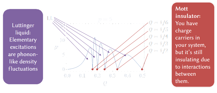
Such a setup causes fermions to stay at least $p$ sites away from each other, otherwise, a huge energy penalty is caused $t\ll U_m$. We can then consider changing the density of the fermions in the system. This causes the emergence of two phases (see Fig. 1):
- Luttinger liquid phase – where elementary excitations are phonon-like density fluctuations – happens for almost all densities $Q$, and
- Mott insulating phase – where despite a presence of the charge carriers the system is insulating due to their repulsive interactions – present only for critical densities $Q_c=1/k$.
Solving the generalised t-V model
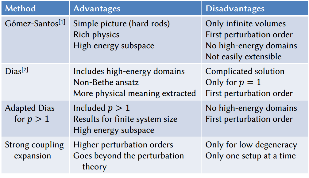
We are interested in solving the generalised $t$-$V$ model by using already-existing analytical tools, such as Gómez-Santos [1] method or the Dias method [2]. We have adapted the Dias method in order to expand the considered interaction range beyond $p=1$. We have also used strong coupling expansion – a method widely used in lattice field theory community – in order to achieve high-perturbation-order estimates of the system near the Mott insulating densities.
We present a short comparison of the methods below in Table 1.

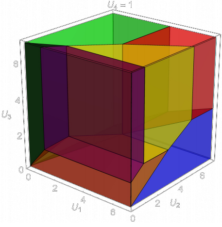
Charge-density-wave phases in the model with unusual potentials
If one considers the potential energy not to be steadily decreasing, the model can exhibit non-trivial behaviour and the emergence of unusual charge-density-wave phases [3,4]. An example phase diagram is shown in Fig. 2 with corresponding phases described in Table 2.
| System | GS unit cell | Energy density | $f$ | |
| $p=4$ $Q=1/3$ $L_\text{max}=36$ | $\vphantom{1\over3}{\bullet}{\circ}{\circ}$ $\vphantom{1\over3}{\bullet}{\bullet}{\circ}{\circ}{\circ}{\circ}$ $\vphantom{1\over3}{\bullet}{\circ}{\bullet}{\circ}{\circ}{\circ}$ $\vphantom{1\over3}{\bullet}{\bullet}{\circ}{\circ}{\circ}{\bullet}{\circ}{\circ}{\circ}$ $\vphantom{1\over3}{\bullet}{\circ}{\bullet}{\circ}{\bullet}{\circ}{\circ}{\circ}{\circ}$ $\vphantom{1\over3}{\bullet}{\circ}{\bullet}{\circ}{\circ}{\bullet}{\circ}{\bullet}{\circ}{\circ}{\circ}{\circ}$ $\vphantom{1\over3}{\bullet}{\bullet}{\bullet}{\circ}{\circ}{\circ}{\circ}{\bullet}{\circ}{\bullet}{\circ}{\circ}{\circ}{\circ}{\bullet}{\circ}{\bullet}{\circ}{\circ}{\circ}{\circ}$ | ${1\over3}U_3$ ${1\over6}U_1$ ${1\over6}(U_2+U_4)$ ${1\over9}(U_1+2U_4)$ ${1\over9}(2U_2+U_4)$ ${1\over12}(2U_2+U_3)$ ${1\over21}(2U_1+3U_2)$ | $\vphantom{1\over3}3$ $\vphantom{1\over3}6$ $\vphantom{1\over3}6$ $\vphantom{1\over3}9$ $\vphantom{1\over3}9$ $\vphantom{1\over3}12$ $\vphantom{1\over3}21$ | $\vphantom{1\over3}{\blacksquare}$ $\vphantom{1\over3}{\blacksquare}$ $\vphantom{1\over3}{\blacksquare}$ $\vphantom{1\over3}{\blacksquare}$ $\vphantom{1\over3}{\blacksquare}$ $\vphantom{1\over3}{\blacksquare}$ $\vphantom{1\over3}{\blacksquare}$ |
$\,$
$\,$
$\,$
References
[1] Gómez-Santos, Phys. Rev. Lett. 70(24), 3780 (1993).
[2] Dias, Phys. Rev. B 62, 7791 (2000).
[3] P. Schmitteckert and R. Werner, Phys. Rev. B 69, 195115 (2004).
[4] T. Mishra, J. Carrasquilla, and M. Rigol, Phys. Rev. B 84, 115135 (2011).