The Schwinger model – what is it?
The Schwinger model is a model of 1+1-dimensional (one spatial and one temporal dimension) of quantum electrodynamics. It describes interacting spin-half particles in an electric field. The model is usually used as a toy model for quantum chromodynamics (QCD), due to its rich physics and similarities to QCD, namely quantum confinement and chiral symmetry breaking.
The lattice formulation
One can represent the Schwinger model on a lattice using staggered fermions. The Hamiltonian is:
$$
H =\, – \frac{i}{2a} \sum_{n=1}^M (\phi_n^\dagger\, e^{i\theta_n}\, \phi_{n+1} – \text{h.c.})+m\sum_{n=1}^M (-1)^n\, \phi_n^\dagger\, \phi_n+\frac{g^2 a}{2} \sum_{n=1}^M (L_n+\alpha)^2
$$
where $a$ is the lattice constant, $M$ is the lattice size, $m$ is the fermion mass, and $g$ is the coupling. $\phi_n$ are the fermionic operators on site $n$, $L$ is the electric field, $\theta$ is related to the electric potential and $\alpha$ is the background electric field. Using the Jordan-Wigner transformation we can change the fermionic picture to boson algebra. The Hamiltonian becomes:
$$
H = \frac{1}{2a} \sum_{n=1}^M (\sigma^+_n \, e^{i\theta_n} \, \sigma^-_{n+1} + \text{h.c}) + m \sum_{n=1}^M (1+(-1)^n \sigma_n^z) + \frac{g\,a^2}{2} \sum_{n=1}^M (L_n+\alpha)^2
$$
where $\sigma$ are the Pauli matrices. The model consists of two degrees of freedom: the spin-half algebra and infinite ladder space of $L$. Therefore, although the system is considered on a finite lattice it has an infinite basis.
Summary of the results
Using strong coupling expansion with exact diagonalisation, we have determined the scalar and vector masses of the model, as shown in Fig. 1.
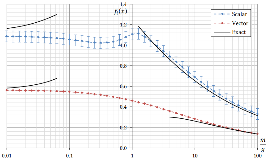
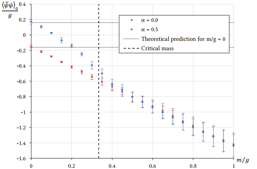
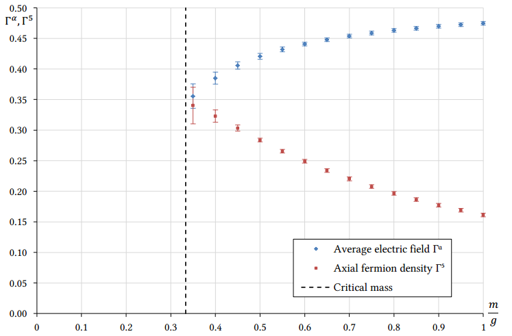
Our results are consistent with theoretical predictions in various limits. In order to show the chiral symmetry breaking, we have determined chiral order parameter (chiral condensate, see Fig. 2) and other parameters that change discontinuously during the symmetry breaking (see Fig. 3). All the computer quantities show discontinuity at the critical fermion mass, which is an indication of chiral symmetry being broken.
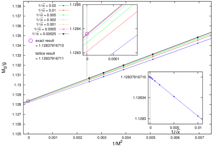
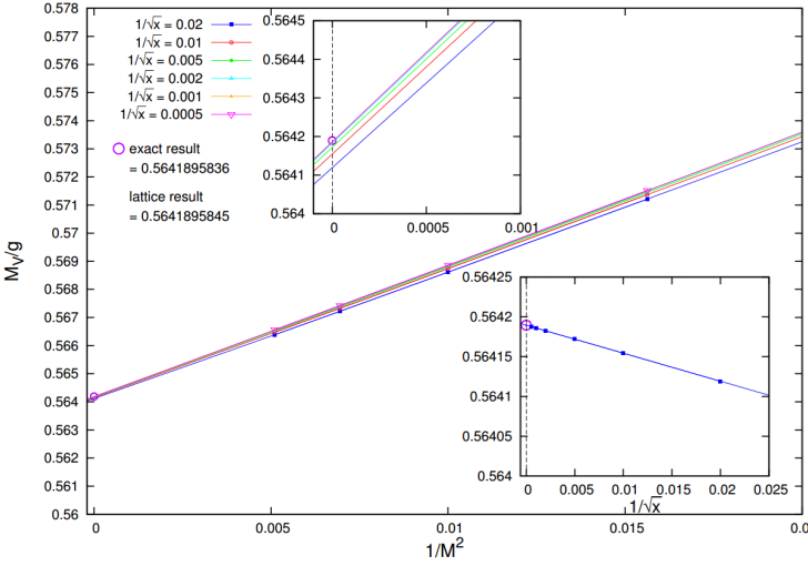
Investigating the model almost at the continuum limit
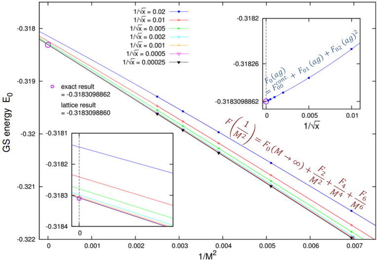
By increasing the strong coupling expansion perturbation order to an extremely high value, one can obtain results, which are saturated up to the computer precision. Then, we perform an extrapolation to infinite volume limit and zero lattice spacing. This gives us estimates for the ground state energy and the scalar and vector mass gaps, which have a staggering precision of 10-11 digits (see Figs. 4-6).
Oscillations of the observables in the strong coupling expansion
If one increases the perturbation order, some observables exhibit an oscillation (see Fig. 7). We believe this to be an artefact of not including enough flux in the calculation. Oscillations clearly have a periodicity of the system size, and one notices that every time a period is finished one more flux loop is present in the system.
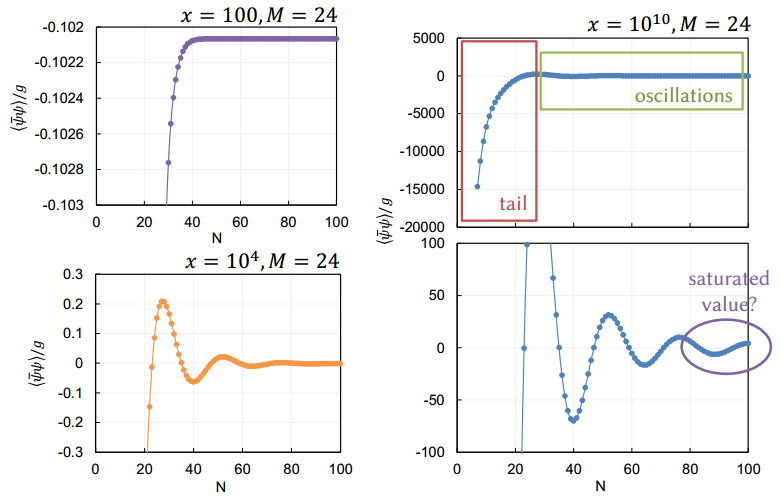
To extract the saturated value, we propose using an oscillatory fit function of the form:
$$
\Sigma(N,M,x) = \Sigma(N\to\infty,M,x)+\left(A(M)\,\frac{x}{N^3} + B(M,x) \,e^{-\alpha(M,x)\, N}\right) \sin \frac{2\pi}{M}(N+1)
$$
where $A(M)$, $B(M,x)$, and $\alpha(M,x)$ are fitting parameters.